Autoregressive Spectral Estimation for detection of short lasting episode of central fixation

Purpose: The birefringent properties of the Henle fibers surrounding the fovea have been used to identify the position of the fovea and the direction of gaze. This allows checking for eye alignment and strabismus - a risk factor for amblyopia. Screening techniques have been reported, based on the birefringence signal derived from foveal circular scanning. The polarization-changing property (birefringence) of the Henle fibers surrounding the fovea has been used to identify its position and hence the direction of gaze [1-5]. Screening techniques and an instrument have been reported, based on the birefringence signal derived from circular scanning in the foveal region [6]. A signal s(t) consisting of several frequency components (f₁=k₁*f_s, f₂=k₂*f_s, f₃ =k₃*f_s, etc) is produced, where each frequency is a multiple of the scanning frequency f_s. Some frequencies prevail during cental fixation, while others appear at paracentral fixation. The existence and the mixture of frequencies depends on the opto-mechanical design. In the simplest case, discussed here, f₂=2f_s is produced during central fixation, while f₁=f_s prevails during off-central fixation. Existing instruments acquire consecutive epochs of s(t), with gaps between them, during which FFT is performed. The problem is that the FFT power spectrum tells how much of f₁ and f₂ are represented in the whole epoch analyzed, but it does not tell exactly where these frequencies appear and for how long. With less-cooperative patients, important short lasting moments of central fixation (f₂) may be hidden behind large low-frequency (f₁) components. Analyzing short time intervals is advantageous, but this is where FFT becomes prone to noise and loses spectral resolution.

Methods: Autoregressive (AR) spectral estimation is proposed to analyze short-lasting non-stationary segments of the scanning signal. AR has an advantage over FFT that, it uses shorter records and has better spectral resolution at that scale.

Apparatus and data

The principle of RBS for the purpose of detecting central fixation has been reported elsewhere [2, 3, 6]. In short, a scanning beam of linearly polarized light is used to circularly scan around the predicted center of the fovea, when the eye is looking at a given central target. The fovea changes the polarization state of light depending on the location of the projection of the spot being scanned (Figure 1). A typical bow-tie pattern (“polarization cross”) exists, created by the radial array of fine Henle fibers which connect the center of the fovea to the optic nerve. The dotted circles on Figure 1 show two possible paths of the stationary circular scan with respect to the center of the fovea, which moves with the eye. Depending on the region on the polarization cross being scanned, the retro-reflected signal can be of two main frequencies.  Moments of central fixation, when the centers of the scanning circle and the fovea coincide, are characterized by dominant frequencies f₂=2f_s   whereas off-central fixation is represented by  f₁=f_s, with  f_s  being the scanning frequency. A typical time-frequency distribution obtained with this type of scanning is shown in Figure 2, where fixation shifts from central to paracentral as time progresses.  The hardware for obtaining the RBS signal is shown in Figure 3, and has been explained in more detail in [6, 7]. Linearly polarized near-infrared (NIR) light of 785 nm wavelength is sent through a non-polarizing beamsplitter to a scanning system, which converts the stationary beam into a circular scan (of scanning frequency 96 rounds per second) subtending an angle of approximately 3⁰ at the subject’s eye. By the eye’s own optics, the beam is focused onto the retina, with the eye fixating on a target appearing at the center of the scanning circle. Upon reflection from the ocular fundus, the polarization-altered light follows the same path back and arrives at the non-polarizing beamsplitter, which deflects part of it toward a polarization analyzing unit. The latter consists mainly of a polarizing beamsplitter, which separates the light into two orthogonal components. The vertical polarization component (s) is reflected, while the horizontal polarization component (p) is transmitted. Each component is captured by a photodetector (PD1 and PD2, respectively) and amplified, then the difference of the two is built in hardware, yielding the S₁ component of the Stokes vector. The signal is then filtered, amplified, and digitized by an analog-to-digital converter (ADC) at a sampling rate of 10 kHz. Scanning signals were recorded from six subjects after obtaining written informed consent, following a protocol approved by the Institutional Review Board (IRB) and in compliance with the Helsinki Declaration. Personal identification data was not collected. From each subject, twelve records were acquired, each 400 ms long, for both the right eye and the left eye. The original device used was binocular [6], but since this work focuses on the signal analysis part, only a monocular implementation was considered.

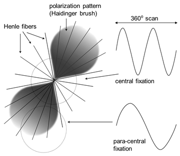
Fig. 1

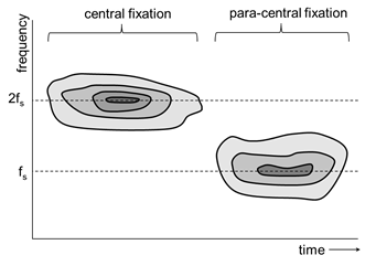
Fig. 2

Autoregressive Spectral Estimation

In the original version of the above described device, the Fast Fourier Transform (FFT) was employed to detect appearances of   f_s=96 Hz and  2f_s =192 Hz. Since the frequency resolution is the reciprocal of the time interval  T  being analyzed, the needed frequency resolution of 96 Hz would require  T  to be not less than 10.4 ms. This, however, would impede the detection of very short lasting episodes (sometimes 5-10 ms), which have been observed in the signal [8].  In addition, because the FFT assumes periodicity, spectral leakage occurs with it due to signal discontinuity. Using a weighting window in an attempt to reduce such leakage also decreases the FFT’s frequency resolution.

Autoregressive (AR) spectral estimation was employed to analyze short-lasting segments of the RBS signal, as an alternative to the FFT. The method has an advantage over FFT that, it can use epochs of shorter duration at sufficient spectral resolution.  The AR methods [9-13] enable representation of a signal in a time interval by means of a set of parameters, namely the autoregressive coefficients:

                                                (1)

in which x(n) is the output sequence of a causal filter that models the observed data, and u(n) is the input driving sequence.  If all moving average parameters b(k) are zero, except b(0)=1, then

                                                                       (2)

is strictly an autoregressive process of order p that allows for the calculation of the power spectrum density (PSD) in an unequivocal manner.  For each signal segment x(n) being analyzed, once the AR parameters have been estimated, the PSD can be computed as:

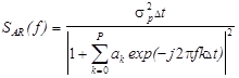                                                                              (3)

where  f  is a frequency contained in the signal being modeled, P is the order of the AR process, a_k   are the AR coefficients, s²_p  is the forward prediction error energy, and Dt is the sampling period of the data sequence. The order determines the trade-off between resolution and estimate variance in AR spectra. The optimum order of the AR model was determined using the Akaike Information Criterion [14].  To find the AR parameters a_k, different methods can be used, such as Yule-Walker, Burg, Covariance method, Modified covariance method, and others. For the purpose of this study, after experimentation on real subjects’ data, the Burg Maximum Entropy method [10, 15, 16] proved to be the most suitable one. This method is based on the extrapolation of the known values of the autocorrelation function (or estimate) using the AR model as the basis for such extrapolation. Assuming that p+1 values of the autocorrelation function R_xx(0)  to  R_xx(p) are known as

with  N  being the total number of points,    (4)

then the maximum entropy extrapolation of the autocorrelation is:

    for |n| > p                                                        (5)

In this equation, two indices are used for the AR coefficients  a(p,k).  The first is the order of the AR model, and the second, the number of the coefficient. In fact, what is being used in (5) is the important property that a coefficient of an AR process  can be computed recursively from the parameters of an AR process (k-1) and the  k  values of the autocorrelation function (Levinson-Durbin algorithm):

from Yule-Walker equations [10]     (6a)

                                                                                      (6b)

Further, consecutive superior orders from  k=2  to  p  are computed as:

                               (7a)

                                                             (7b)

                                                                                 (7c)                                                                   

Where s² is the variance of the driving white noise. Once the desired order  p  is reached, the PSD is estimated according to equation (3) above.  Alternatively, knowing the maximum entropy extrapolations from equation (5) and using equations (6a) through (7c), the PSD equivalent to (3) can be expressed directly in terms of the maximum entropy extrapolation of the autocorrelation:

                                                                    (8)

In the above formula,  M  can be chosen as a power of two, in order to allow computation using an FFT.  In this study, both M=8 and M=16 gave good results.  Equations (3) and (10) produced the same PSD and performed approximately at the same speed.

The Burg maximum entropy method minimizes the randomness (entropy) of the unknown time series, producing the flattest (“whitest”) spectrum of all the alternatives for which the autocorrelation function in the interval  r_xx(0)  to  r_xx(p)  is equal to the known lags R_xx(0)  to  R_xx(p) [16]. Another advantage is that the maximum entropy extrapolation imposes the fewest constraints on the unknown time series [10]. This method also minimizes the sum-squared of the forward and backward prediction errors and has minimal phase characteristics. 

To determine whether the model actually fits the data, the residuals between the true values and predicted values at each sample were computed. A good AR model is indicated by the residuals being a white noise process. The whiteness of the residuals was tested using the cumulative periodogram method [9]. All tests passed for a model order of  p = 16…21.

Results: Figure 1 below illustrates the AR-based analysis during central fixation (left column), and lack thereof (right column). The upper row shows the time domain scan signal (5 ms, scanning frequency f_s=96 Hz, sampling rate SR=10 kHz). The middle row is the FFT power of the same signal, having a spectral resolution of 200 Hz. The lower row shows continuous AR power spectral densities, capable of detecting intermediate frequencies.
Conclusions: AR spectral estimation is superior to FFT in analyzing short segments. With modern DSP technology, it can be performed fast, thus reducing signal gaps while increasing temporal resolution.

 References

[1] Hunter DG, Patel SN, Guyton DL. Automated detection of foveal fixation by use of retinal birefringence scanning. Appl Optics. 1999;38:1273-9.

[2] Guyton DL, Hunter DG, Patel SN, Sandruck JC, Fry RL. Eye Fixation Monitor and Tracker.  US Patent No 6,027,2162000.

[3] Gramatikov BI, Zalloum OH, Wu YK, Hunter DG, Guyton DL. Birefringence-based eye fixation monitor with no moving parts. J Biomed Opt. 2006;11:34025.

[4] Irsch K, Gramatikov BI, Wu YK, Guyton DL. New pediatric vision screener employing polarization-modulated, retinal-birefringence-scanning-based strabismus detection and bull's eye focus detection with an improved target system: opto-mechanical design and operation. J Biomed Opt. 2014;19:067004.

[5] Gramatikov BI. Modern technologies for retinal scanning and imaging: an introduction for the biomedical engineer. Biomedical engineering online. 2014;13:52.

[6] Hunter DG, Nassif DS, Piskun NV, Winsor R, Gramatikov BI, Guyton DL. Pediatric Vision Screener 1: instrument design and operation. J Biomed Opt. 2004;9:1363-8.

[7] Gramatikov B, Irsch K, Mullenbroich M, Frindt N, Qu Y, Gutmark R, et al. A device for continuous monitoring of true central fixation based on foveal birefringence. Ann Biomed Eng. 2013;41:1968-78.

[8] Gramatikov B. Detecting fixation on a target using time-frequency distributions of a retinal birefringence scanning signal. Biomedical engineering online. 2013;12:41.

[9] Box GEP, Jenkins GM. Time Series Analysis: Forecasting and Control. Oakland, California: Holden-Day; 1976.

[10] Kay SM, Marple SL. Spectrum analysis - A modern perspective. Proc IEEE. 1981;69(11):1380-419.

[11] Kay SM. Modern Spectral Estimation, Theory and Application. New Jersey: Prentice Hall, Englewood Cliffs; 1988.

[12] Marple SL. Digital Spectral Analysis with Applications. New Jersey Prentice Hall, Englewood Cliffs; 1987.

[13] Akay M. Biomedical signal processing. San Diego, CA: Academic Press, Inc.; 1994.

[14] Akaike H. A new look at the statistical model identification. IEEE Trans Automatic Control. 1974;AC-19:716-23.

[15] Burg JP. Maximum entropy spectral analysis [Ph.D.]. Stanford, CA: Stanford University; 1975.

[16] Schlindwein FS, Evans DH. A real-time autoregressive spectrum analyzer for Doppler ultrasound signals. Ultrasound in medicine & biology. 1989;15:263-72.

The above material has been published in full in the following paper:

Gramatikov, B. I. Detection of central fixation using short-time autoregressive spectral estimation during retinal birefringence scanning. Medical Engineering & Physics (Elsevier), September 2015, 37(9), pp. 905–910; 10.1016/j.medengphy.2015.06.007.

http://dx.doi.org/10.1016/j.medengphy.2015.06.007