Using an artificial neural network to detect central fixation and eye alignment, to identify risk factors for amblyopia
For a more detailed version of this research report, please read the following publication:
Gramatikov, B.I. Detecting central fixation by means of artificial neural networks in a pediatric vision screener using retinal birefringence scanning. BioMedical Engineering OnLine (Springer), April 2017.
Amblyopia (“lazy eye”) is poor development of vision from prolonged suppression in an otherwise normal eye, and is a major public health problem, with impairment estimated to afflict up to 3.6% of children – and more in medically underserved populations [1]. Reliable detection of eye alignment with central fixation (CF) is essential in the diagnosis of amblyopia. Further, there is a need for a commercially available and widely accepted automated screening instrument that can reliably detect strabismus and defocus in young subjects [2]. Our laboratory has been developing novel technologies for detecting accurate eye alignment directly, by exploiting the birefringence (a property that changes the polarization state of light) of the uniquely arranged nerve fibers (Henle fibers) surrounding the fovea. We employed retinal birefringence scanning (RBS), a technique that uses the changes in the polarization of light returning from the eye, to detect the projection into space of the array of Henle fibers surrounding the fovea [3-5]. In RBS, polarized near-infrared light is directed onto the retina in a circular scan, with a fixation point in the center, and the polarization-related changes in light retro-reflected from the ocular fundus are analyzed by means of differential polarization detection. Due to the radially symmetric arrangement of the birefringent Henle fibers, a characteristic frequency appears in the obtained periodic signal when the scan is centered on the fovea, indicating central fixation. By analyzing frequencies in the RBS signal from both eyes simultaneously, the goodness of eye alignment can be measured, and thus strabismus (misaligned eyes) can be detected. RBS technology is the only known technology that can detect central fixation remotely using true anatomical information (position of the fovea). An early version of the “Pediatric Vision Screener” (PVS) was designed in our lab and then tested at the Boston Children’s Hospital, [6-10]. This prototype device has been developed into a commercial instrument that detects eye alignment (REBIScan, Boston, MA).
Meanwhile, development of the RBS technology has continued in our lab, resulting in a series of central fixation detecting devices with no moving parts [11, 12], devices for continuous monitoring of fixation [13], a device for biometric purposes [14], and ultimately an improved PVS that combines “wave-plate-enhanced RBS” [15], or “polarization-modulated RBS” [16, 17], for detecting strabismus, with added technology for assessing proper focus of both eyes simultaneously. Polarization-modulated RBS is an optimized upgrade of RBS, based upon our theoretical and experimental research and computer modeling, using a spinning half wave plate (HWP) and a fixed wave plate (WP) to yield high and uniform signals across the entire population. In addition, using a technique named “phase-shift-subtraction” (PhSS), the new PVS eliminated the need for initial background measurement [15-17].
Depending on the direction of gaze and the design of the instrument, the screener produces several signal frequencies that can be utilized in the detection of central fixation. Using a computer model involving all polarization-changing components of the system, including the Henle fibers and the cornea, we found that by spinning the HWP 9/16-ths as fast as the circular scan, strong signals are generated that are odd multiples of half of the scanning frequency [17]. With central fixation, two frequency components predominate the RBS signal: 2.5 or 6.5 times the scanning frequency fs, depending on the corneal birefringence. With paracentral fixation, these frequencies practically disappear, being replaced by 3.5fs and 5.5fs. Therefore, the relative strengths of these four frequency components in the RBS signal distinguishes between central and paracentral fixation. In addition, a strong, spin-generated, 4.5fs frequency in our RBS signal that is practically independent of corneal birefringence and of the position of the scanning circle with respect to the center of the fovea [16]. This “spin-generated frequency” is thus well suited for normalization of the signal, in order to limit the subject-to-subject variability.
The PVS instrument design has been described in detail elsewhere, and encouraging results have been reported [16-18]. We validated the performance of this research instrument on an initial group of young test subjects – 18 patients with known vision abnormalities (8 male and 10 female), ages 4-25 (only one above 18), and 19 control subjects with proven lack of vision issues. Four statistical methods were used to derive decision making rules that would best separate patients with abnormalities from controls. Method 1 (termed “Simple threshold”) employed gradual changing of an adaptive threshold θ for the normalized combined power at CF frequencies (P2.5+P6.5)/ P4.5 , in order to minimize the classification errors. Methods 2, 3 and 4 employed linear discriminant analysis, basically using a linear combination of respectively 2, 3 or 4 features (in our case normalized signal powers at different frequencies) to separate the two classes (CF vs para-CF). Ultimately, classification is based on a linear classifier involving the coefficients of a 2-, 3- or 4-way discriminant function. Sensitivity and specificity were calculated for each method [18]. The discriminant functions methods provided excellent specificity of 100%, but relatively low sensitivities of 90% or below. This meant that although all detected abnormalities would be true, at least 10% of the children with strabismus would be missed. For this reason we chose the “Simple threshold” (Method 1) which on the calibration data gave sensitivity of 99.17% and specificity of 96.25%.
The objective of the present study was, based on the characteristic signal frequencies mentioned above, to develop and test an Artificial Neural Network (ANN) for the detection of central fixation, and to compare it with the classical statistical methods, reported earlier.
Artificial neural networks have quite often been used for diagnostic purposes in the past two-three decades. Applications include the diagnosis of myocardial infarction [19], waveform analysis of biomedical signals, medical imaging analysis and outcome prediction [20], automatic detection of diabetic retinopathy [21], nephritis and heart disease [22], biochemical data and heart sounds for valve diagnostics [23], and many more. There are reports in the literature relating to the use of artificial neural networks for eye tracking [24-28]. They are mostly used as part of a human-computer interface, or as an aid for the handicapped, and work typically with a camera which tracks the pupil using either infrared or visible light images of the pupil. Through proper training, neural networks can provide precise individual calibration. Such networks often employ on the order of 20 to 200 dimensions (hidden neurons), and can require significant computing time. They are accurate to approximately 0.75˚. In our application, the signals are available as spectral powers at just a few frequencies, generated upon retinal birefringence scanning around the fovea. They allow the detection of central fixation with much higher precision (0.1˚) without the need for full-range eye tracking or calibration, while allowing some head mobility. Applications of artificial neural networks for this purpose are unknown to the author.
The optics, electronics, and signal analysis of the PVS have been reported in more detail previously [16-18]. This present work focuses on the use of artificial neural networks as an alternative to classical statistical methods. The goal of this study was, if possible, to improve the classification algorithms, as well as to validate the performance of the research instrument on the same group of young test subjects that was used in the previous study, with the addition of two more subjects. All subjects’ data were analyzed with both the methods from the previous paper, and the neural networks method reported here. For more detail on the human subject data, please see the Data section below. The neural network performance is compared with the four statistical methods that were applied to the same dataset earlier, and the ability to separate patients with abnormalities from controls was investigated.
Artificial neural networks
Artificial neural networks have been widely used, and the related theory has matured in the last three decades [29-35]. Feedforward neural networks (FNNs) are static, i.e. networks with no feedback elements and no delays. They are widely used to solve complex problems in pattern classification, system modeling and identification, and non-linear signal processing, and in analyzing non-liner multivariate data. One of the characteristics of the FNN is its learning (or training) ability [36]. It has a learning process in both hidden and output layers. By training, the FFNs can give correct answers not only for learned examples, but also for the models similar to the learned examples, showing their strong associative ability and rational ability which are suitable for solving large, nonlinear, and complex classification and function approximation problems. The classical method for training FNNs is the backpropagation (BP) algorithm [31] which is based on the gradient descent optimization technique.
Many tools have been developed for creating and testing ANN networks. Among them, probably the most significant one is the Neural Networks Toolbox for MATLAB from MathWorks, Inc. [37] The author employed this toolbox for creating, training, and testing the network with both calibration and clinical data. Another useful tool widely used in the field is the Netlab simulation software, designed to provide the central tools necessary for the simulation of theoretically well-founded neural network algorithms for use in teaching, research, and applications development. It consists of a library of MATLAB functions and scripts based on the approach and techniques described in the book Neural Networks for Pattern Recognition by Dr. Christopher Bishop [38], Department of Computer Science and Applied Mathematics at Aston University, Birmingham, UK.
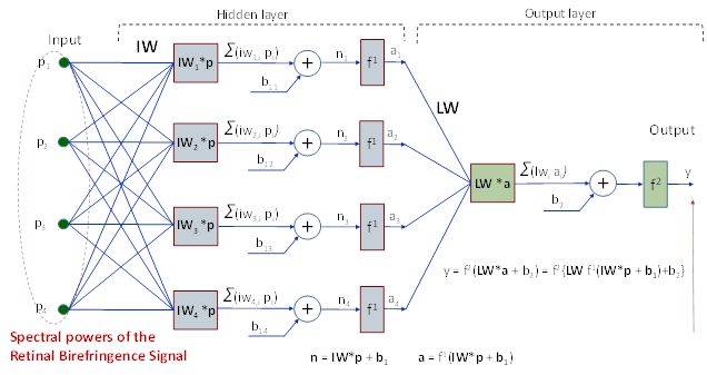
Figure 1. Neural network architecture. A two-layer architecture has been employed, consisting of one hidden layer and one output layer. The network has an input p containing four inputs (p1 to p4), representing the four normalized RBS spectral powers, respectively P2.5/P4.5, P3.5/P4.5, P5.5/P4.5, and P6.5/P4.5. The hidden layer contains four neurons. The output of the net signals presence or absence of central fixation.
Neural Network Architecture
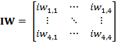
For the present application, several ANN architectures were tested. To avoid overfitting (explained later under Generalization), a relatively simple architecture was selected (Figure 1), consisting of one hidden layer and one output layer. This two-layer network has an input p containing four inputs (p1 to p4), representing the normalized RBS spectral powers, respectively P2.5/P4.5, P3.5/P4.5, P5.5/P4.5, and P6.5/P4.5, that are generated during retinal birefringence scanning. The hidden layer contains four neurons. Each neuron is connected to each of the inputs through the input weight matrix IW:
 (1)
(1)
The i-th neuron has a summer that gathers its weighted inputs iwi,j and a bias b1,i, to form its scalar output ni as:
ni = iwi,1p1 + iwi2p2 + iwi,3p3 + iwi,4p4 + b1,i (2)
equivalent to a dot-product
(inner product):
![]() (3)
(3)
Where b1 is a four-element vector representing the four biases, one for each neuron.
Each ni
then is processed by a sigmoid transfer function f1 to
deliver a neuron output ai. The 4-element output vector of the
four neurons (and the hidden layer as a whole) can be represented in matrix
form as:
![]() (4)
(4)
The four neuron outputs are then fed to the output layer, which has a neuronal structure as well. Its scalar output y can be represented by the equation
y = f2(LW*a + b2) = f2{LW f1(IW*p + b1) + b2} (5)
where LW is the output layer weight matrix and the scalar b2 is the output neuron’s bias:
LW = [ lw1 lw2 lw3 lw4 ] (6)
The weights and biases were calculated during the training of the network, as explained later. The sigmoid transfer functions for the hidden layer f1 and for the output layer f2 were chosen to be the same, namely of type Log-Sigmoid transfer function (logsig):
logsig(n) = 1 / (1 + exp(-n)) (7)
The function logsig generates outputs between 0 and 1 as the neuron’s net input goes from negative to positive infinity. As mentioned above, the neural network shown in Figure 1 is a FFN. Feedforward networks consist of a series of layers. The first layer has a connection from the network input. Each subsequent layer has a connection from the previous layer. The final layer produces the network's output. FFNs can be used for any kind of input to output mapping. A feedforward network with one hidden layer, and enough neurons in the hidden layers, can fit any finite input-output mapping problem. It can be used as a general function approximator. It can approximate, arbitrarily well, any function with a finite number of discontinuities, given sufficient a number of neurons in the hidden layer. Specialized versions of the feedforward network include fitting and pattern recognition networks. The pattern recognition networks are the ANN of choice when solving classification problems, such as ours. In pattern recognition problems, we want a neural network to classify inputs into a set of target categories. Thus, pattern recognition networks are FFNs that can be trained to classify inputs according to already verified target classes, in our case verified central fixation versus paracentral fixation.
Creating the Neural Network
Following the above reasoning, our neural network was created (as a network object) using the MATLAB Toolbox’s pattern recognition network creation function patternnet:
net = patternnet(hiddenLayerSize, trainFcn); (8)
The parameter hiddenLayerSize here is 4, corresponding to the four neurons in the hidden
layer. One can change the number of neurons if the network does not perform
well after training, and then retrain. The parameter trainFcn
defines the training function, which in our case is 'trainscg’,
standing for the scaled conjugate gradient backpropagation method for updating weight and bias values during training
[39]. It performed
slightly better on our data than the popular and faster Levenberg–Marquardt
(LM) training algorithm [40].
Backpropagation (explained below) is used to
calculate derivatives of performance perf with respect to the weight and bias variables.
Data
To
define a pattern recognition problem, data is generally arranged in a set of Q
input vectors (measurements) as columns in a matrix. Then another set of Q
target vectors is arranged, so that they indicate the classes to which the
input vectors are assigned. Classification problems involving only two classes
(as in our case) can be represented by target vectors consisting of either
scalar 1/0 elements, which is the format used in this study. Alternatively, the
target could be represented by two-element vectors, with one element being 1
and the other element being 0. In the general case, the target data for pattern recognition networks should consist of
vectors of all zero values except for a 1 in element i,
where i is the class they
represent.
The calibration data were comprised of the same data set that was used in an earlier study [18]. Briefly, with the Pediatric Vision Screener [16-18] we recorded signals from five asymptomatic normal volunteers, ages 10, 18, 24, 29 and 39, two female and three male, of them three Caucasian, one African American, and one Asian, all properly consented. The subjects were asked to look first at the blinking target in the center of the scanning circle, for central fixation (CF). Twelve measurements of duration 1 s were taken in order to obtain representative data while taking into consideration also factors like fixation instability and distractibility. The calculated FFT powers for each measurement were saved on disk. The same type of measurement was repeated with each of the subjects looking at imaginary “targets” on the scanning circle (1.5⁰ off center) at 12, 3, 6, and 9 o’clock. The spacing was chosen such that there would be a sufficient distance between the targets, to avoid confusion in the test subject, and to overcome the natural instability of fixation. More fixation points or more than 12 measurements per target have proven to diminish the efficiency of data collection, because of fatigue occurring in the test subjects. The data, consisting of powers P2.5, P6.5, P3.5, P5.5 and P4.5 for each of the 12 measurements of each eye of all five test subjects, were bundled into two groups: a group for central fixation (120 “eyes,” the “CF set”) and a group for paracentral fixation (480 “eyes,” the “para-CF set”). Data from these two controlled groups were used to create and calibrate the ANN. The data were organized as an input matrix of 4 rows and Q columns, with Q = 600 (120 measurements with CF and 480 measurements with para-CF). The target vector was a vector of length Q=600, each element of which was either 1 (CF) or 0 (para-CF). These inputs and targets were used for training, validation and testing the network. One can reasonably argue that this number of subjects (5) and eyes (10) is insufficient for providing reliable calibration with regard to the two classes (CF vs. para-CF). Yet, the variability of the RBS signals’ waveforms (and respectively the five derived frequency powers) depend to a much higher extent on the subject’s direction of gaze and the ability to fixate, than on the individual variability of the foveal and corneal birefringence. This invariability, especially to corneal birefringence, was achieved with the new design, as reported in our previous work [15-17]. The birefringence of the fovea is largely constant. It is the corneal birefringence that affects the signals. The cornea, acting as a retarder of a certain retardance and azimuth, influences the orientation of the polarization cross. In the design of the PVS [18], the corneal birefringence was compensated for by means of a wave plate (retarder), achieving broad uniformity across the population studied. The wave plate was optimized by means of a dynamic computer model of the retinal birefringence scanning system (including the retina and the cornea as part of a train of optical retarders) and based on the data from a database of 300 eyes [15].
The clinical data were also obtained with the Pediatric Vision Screener (following an institutionally approved IRB protocol), and were almost identical with the data set used in [18], with the addition of just two more subjects, both of whom were independently verified by a pediatric ophthalmologist. Thus, the total was 39 test subjects: 19 properly consented patients with known abnormalities (9 male and 10 female, of which 12 Caucasian, 2 African American, and 5 Asian), ages 4-25 (only one above 18), and 20 control subjects with proven lack of vision issues (10 male and 10 female, of which 16 Caucasian, 1 African American, and 3 Asian), ages 2-37 (only 4 above 18), all properly consented. All were recruited from the patients of the Division of Pediatric Ophthalmology at the Wilmer Eye Institute, or the patients’ siblings. All subjects underwent a vision exam by an ophthalmologist, during which eye alignment and refraction were tested. On the whole, verified information was available from a total of 78 eyes. Data were organized as an input matrix of 4 rows and Q columns (Q = 78 eyes). The target vector was a vector of length Q (Q=78), each element of which was either 1 (CF) or 0 (para-CF). These inputs and targets, as well as the network outputs, were used for testing the performance of the ANN and comparing it to the statistical methods reported earlier [18].
Preprocessing and Postprocessing
Neural network training can be made more efficient if one performs certain preprocessing steps on the network inputs and targets [35, 37]. The sigmoid transfer functions that are generally used in the hidden layers become essentially saturated when the net input is greater than three. If this happens at the beginning of the training process, the gradients will be very small, and the network training will be very slow. It is standard practice to normalize the inputs before applying them to the network. Generally, the normalization step is applied to both the input vectors and the target vectors in the data set. The input processing functions used here are removeconstantrows (removes the rows of the input vector that correspond to input elements that always have the same value, because these input elements are not providing any useful information to the network), and mapminmax (normalize inputs/targets to fall in the range [-1,1]). For outputs, the same processing functions (removeconstantrows and mapminmax) are used. Output processing functions are used to transform user-provided target vectors for network use. Then, network outputs are reverse-processed using the same functions to produce output data with the same characteristics as the original user-provided targets.
Dividing the Data
When training multilayer networks, the general practice is to first divide the data into three subsets. The first subset is the training set, which is used for computing the gradient and updating the network weights and biases. This set is presented to the network during training, and the network is adjusted according to its error. The second subset is the validation set. It is used to measure network generalization, and to halt training when generalization stops improving. The error on the validation set is monitored during the training process. The validation error normally decreases during the initial phase of training, as does the training set error. However, when the network begins to overfit the data, the error on the validation set typically begins to rise. The network weights and biases are saved at the minimum of the validation set error. The test set has no effect on training and so provides an independent measure of network performance during and after training. Test set error is not used during training, but it is used to compare different models. It is also useful to plot the test set error during the training process. If the error on the test set reaches a minimum at a significantly different iteration number than the validation set error, this might indicate a poor division of the data set.
In the Neural Networks Toolbox for MATLAB [37], there are four functions provided for dividing data into training, validation, and test sets. They are dividerand (divide data randomly, the default), divideblock (divide into contiguous blocks), divideint (use interleaved selection), and divideind (divide by index). The data division is normally performed automatically when the network is trained. In this study, the dividerand function was used, with 70% of the data randomly assigned to training, 15% of the data randomly assigned to validation, and 15% of the data randomly assigned to the test set. This is the default partitioning in Neural Networks Toolbox. The appropriateness of this division is discussed in the Discussion and Limitations section below.
Initializing Weights (init)
Before training a feedforward network, one must initialize the weights and biases. The configure command automatically initializes the weights, but one might want to reinitialize them. This is done with the init command. This function takes a network object as input and returns a network object with all weights and biases initialized. Here is how a network is initialized (or reinitialized):
net = init(net); (9)
Performance function
Once the network weights and biases are initialized, the network is ready for training. The training process requires a set of examples of proper network behavior—network inputs p and target outputs t. The process of training a neural network involves tuning the values of the weights and biases of the network to optimize network performance, as defined by the network performance function. The default performance function for feedforward networks is mean square error mse - the average squared error between the network outputs y and the target outputs t [37]. It is defined as follows:
![]() (10)
(10)
For a neural network classifier, during training one can use mean squared error or cross-entropy error, with cross-entropy error being considered slightly better [41]. We tested both methods on a subset of the data, and obtained slightly better results with the cross-entropy method. Which is why the network performance evaluation in this study was done by means of the cross-entropy method:
net.performFcn = 'crossentropy'; (11)
The MATLAB performance function has the following format:
perf = crossentropy(net,targets,outputs,perfWeights)
(12)
It calculates a network performance given
targets (t) and outputs (y), with optional performance weights and other
parameters. The function returns a result that heavily penalizes outputs that
are extremely inaccurate (y near 1-t),
with very little penalty for fairly correct classifications (y near t).
Minimizing cross-entropy leads to good classifiers. The cross-entropy for each
pair of output-target elements is calculated as:
ce = -t .*
log(y)
(13)
where .* denotes element-by-element multiplication. The aggregate cross-entropy performance is the mean of the individual values:
perf = sum(ce(:))/numel(ce)
(14)
In the special case of N = 1 (our case) when the output consists of only one element (y), the outputs and targets are interpreted as binary encoding. That is, there are two classes with targets of 0 and 1. The binary cross-entropy expression is:
ce = -t .* log(y) - (1-t) .* log(1-y)
(15)
where .* denotes element-by-element multiplication.
Training the network
For training multilayer feedforward networks, any standard numerical optimization algorithm can be used to optimize the performance function, but there are a few key ones that have shown excellent performance for neural network training. These optimization methods use either the gradient of the network performance with respect to the network weights, or the Jacobian of the network errors with respect to the weights. The gradient and the Jacobian are calculated using a technique called the backpropagation algorithm, which involves performing computations backward through the network. The backpropagation computation is derived using the chain rule of calculus and is described in more detail in [33] and in [31]. As a note on terminology, the term “backpropagation” is sometimes used to refer specifically to the gradient descent algorithm, when applied to neural network training. That terminology is not used here, since the process of computing the gradient and Jacobian by performing calculations backward through the network is applied in all of the training functions offered by MATLAB’s Neural Networks Toolbox. It is clearer to use the name of the specific optimization algorithm that is being used (i.e. 'trainscg', 'trainlm', 'trainbr', etc.), rather than to use the term backpropagation alone.
Neural networks can be classified into static and dynamic categories. Static networks (which are essentially the FFNs) have no feedback elements and contain no delays; the output is calculated directly from the input through feedforward connections. In dynamic networks, the output depends not only on the current input to the network, but also on the current or previous inputs, outputs, or states of the network. These dynamic networks may be recurrent networks with feedback connections or feedforward networks with imbedded tapped delay lines (or a hybrid of the two) [34]. For static networks, the backpropagation algorithm is usually used to compute the gradient of the error function with respect to the network weights, which is needed for gradient-based training algorithms [42].
The actual training was completed using the function from MATLAB’s Neural Networks Toolbox:
[net,tr] = train(net,x,t) (16)
with x being the input matrix (600 column vectors of size x), and t being the target vector of size 600 (total number of observations in the calibration set).
Network performance was calculated using the perform function
performance = perform(net,t,y) (17)
which takes the network object, the targets t and the outputs y and returns performance using the network's performance function net.performFcn (crossentropy in our case). Note that training automatically stops when generalization stops improving, as indicated by an increase in the cross-entropy error of the validation samples.
Generalization
Neural networks are sensitive to the number of neurons in their hidden layers. Too few neurons can lead to underfitting. Too many neurons can contribute to overfitting, in which all training points are well fitted, but the fitting curve oscillates significantly between these points, and so do the calculated coefficients. In ANN terms, the model does not generalize well. It is apparent from testing with an increasing complexity that as the number of connections in the network increases, so does the propensity to overfit to the data. The phenomenon of overfitting can always be seen as we make our neural networks deep (complex).
In this study, the number of neurons in the hidden layer was chosen empirically. On the clinical data, less than four input neurons did not provide the accuracy achieved with 4-8 neurons in the hidden layer, most likely because of underfitting. At about 10 neurons and upwards, the accuracy started to decrease again, because of overfitting. The choice of 4 hidden neurons was made for two reasons: a) keep the network generalized (i.e. to avoid overfitting), and b) to keep it simple and computationally fast. With respect to the number of hidden layers, no significant improvement was achieved with a two-hidden-layer structure, regardless of the number of neurons in each layer.
MathWorks suggests several ways to improve
network generalization and avoid overfitting [37, 43]. One method for improving network
generalization is to use a network that is just large enough to provide an
adequate fit. The larger network we use, the more complex the functions the
network can create. If a small enough network is used, it will not have enough
power to overfit the data. One can check the Neural
Network Design example nnd11gn in [33] to investigate how
reducing the size of a network can prevent overfitting. Another approach is
retraining. Typically each backpropagation training session starts with
different initial weights and biases, and different divisions of data into
training, validation, and test sets. These different conditions can lead to
quite different solutions for the same problem. Therefore, it is a good idea to
train several networks, in order to ensure that a network with good
generalization is found.
The default method for improving generalization is the so-called early stopping. This technique is automatically provided for all of the supervised network creation functions in the Neural Networks toolbox, including the backpropagation network creation functions such as feedforwardnet and patternnet. As explained before, in this technique the available data are divided into three subsets. The first subset is the training set, which is used for computing the gradient and updating the network weights and biases. The second subset is the validation set. The error on the validation set is monitored during the training process. The validation error normally decreases during the initial phase of training, as does the training set error. However, when the network begins to overfit the data, the error on the validation set typically begins to rise. When the validation error increases for a specified number of iterations (net.trainParam.max_fail), the training is stopped, and the weights and biases at the minimum of the validation error are returned. The test set error is not used during training, but it is used to compare different models. It is also useful to plot the test set error during the training process. If the error in the test set reaches a minimum at a significantly different iteration number than the validation set error, this might indicate a poor division of the data set [43].
There is yet another method for improving generalization, called regularization. It involves modifying the performance function, which is normally chosen (mse, cross-entropy, or other). Using a modified performance function causes the network to have smaller weights and biases, forcing the network response to be smoother and less likely to overfit [43]. Regularization can be done automatically by using the Bayesian regularization
training function trainbr. This can be done by setting net.trainFcn to `trainbr'. This will also automatically move any data in the validation set to the training set [37].
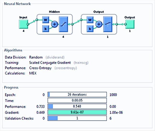
Figure 2. Neural network training tool (nntraintool) representing the training process. The upper part illustrates the network architecture, as shown in Figure 1, this time generated by MATLAB. Training was stopped after iteration 26, at performance 0.548.
Results
Network creation and training
The neural network was trained, validated, and tested on the calibration data of 600 eyes (explained in more detail under the Data subsection in Methods above). Figure 2 shows the NN training process (nntraintool). The upper part illustrates the network architecture, as shown in Figure 1, this time generated by MATLAB. The tool shows the algorithms used, as well as the training progress. Training was stopped after iteration 26, at performance 0.548. Figure 3 shows the dynamics of the training state in terms of gradient of the cross-entropy, on a logarithmic scale. At the endpoint, the gradient was 9.6137x10⁻⁷, which can be considered a good value at which to stop for this set of data.
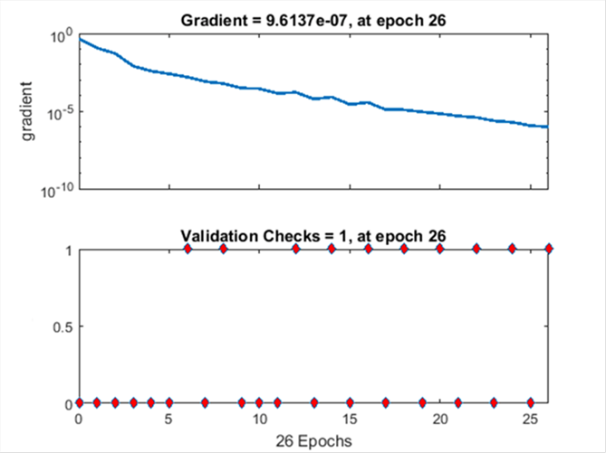
Figure 3. Dynamics of the neural network training state in terms of gradient of the cross-entropy, on a logarithmic scale. At the endpoint, the gradient was 9.6137x10⁻⁷.
Overall, 100.0 % of the predictions are correct and there are no wrong classifications. In terms of sensitivity and specificity, this corresponds to sensitivity=100.0% and specificity=100.0% (Table 1), and exceeds the results from our previous study [18], where none of the statistical methods applied to the same data reached this accuracy (please see columns CAL in Table 1). The reader should, however, be reminded, that this was achieved at a relatively small size of the training set, with the data having been provided by just 10 eyes from 5 patients.
Weights and biases of the ANN
After initialization and training, the weights for the hidden layer, contained in matrix IW, according to (1) above, and as extracted with MATLAB function cell2mat(net.IW), were:
IW =
[ 0.8343 -1.6768 0.3476 0.8698
-1.5320 1.3417 1.8045 -1.9192
-1.0271 0.6329 1.4755 -1.2509
-2.3183 0.6270 3.2967 -5.0483 ]
The bias vector for the hidden layer, as accessed with function cell2mat(net.b(1)), was
b1 = [ -1.6671 -0.1457 -0.0155 -2.3648 ]
The output weights LW, as accessed with MATLAB function cell2mat(net.LW), were
LW = [ 1.5379 -2.9153 -1.8245 -11.3109 ]
Finally, the output bias, b2 = cell2mat(net.b(2)), a scalar, was
b2 = 0.3771
It should be noted that because of the random assignment of the data (training, validation, and test sets), the above weights and coefficients may vary somewhat. This, however, did not impact the sensitivity and specificity significantly. Nevertheless, we trained and retrained the network four times. With all four sessions, both the sensitivity and specificity for the calibration data remained 1.000. For the clinical data, the results from the session which maximized the sensitivity were chosen, because the main goal of this project was to develop a screening device for children, which should not miss lack of central fixation.
Networks with more neurons in the hidden layer, as well as networks with two hidden layers were also tested on the calibration dataset, but they did not improve performance. Their use was avoided because of the risk of potential overfitting.
Testing the ANN on the clinical data
Once the neural network was created, trained, validated, and tested on the calibration data, in a further step, it was tested on our data set of clinical data (described in detail above under the Data subsection in Methods) consisting of a subset of strabismic eyes and a control subset of normal eyes, all obtained with the Pediatric Vision Screener. Four normalized spectral powers from a total of 78 eyes were organized as an input matrix of 4 rows and Q columns (Q = 78). The target vector was a vector of length 78, each element of which was either 1 (CF) or 0 (para-CF). The four inputs for each subject were fed to the ANN, and the output was compared each time with the target, which in fact was the doctor’s decision. This allowed the calculation of the sensitivity and specificity of the ANN when applied to the clinical data. Further, these results permitted a comparison between the performance of the ANN and the statistical methods reported earlier [18], such as the simple adaptive threshold that minimized the overall error, or 2-, 3- and 4-way linear discriminant analysis. The results are summarized in Table 1, columns SBJ (human subjects). The two new patients (4 eyes) were quite “tricky” adding two false negative decisions to the “Standard Threshold” method and just one false negative decision to the neural network’s results. Again, the ANN performed slightly better than the other methods, with sensitivity of 0.9851 and specificity of 1.0000, with no false positive decisions and only one false negative decision. Generally, the discriminant-analysis-based methods showed lower sensitivity. Specificity on the clinical data was 1.0000 for all methods except for the 2-way discriminant analysis. Note that the only other method that used all four inputs separately is the 4-way discriminant analysis, giving a sensitivity of 0.9417 for the calibration data, and only 0.8507 for the clinical data. The excellent performance of the ANN is obviously due to the two-layer structure and to the nonlinear (sigmoid) transfer function at the output of each neuron, giving more flexibility, while the performance of all discriminant functions used in the previous study was strictly linear, resembling just one layer of neurons with a linear transfer function, not ideal for pattern recognition.
Table 1. Performance of the artificial neural network compared with statistical methods with regard to classifying fixation as central versus paracentral fixation
|
|
Neural Network |
Simple threshold |
Discriminant Analysis |
|||||||
|
2D |
3D |
4D |
||||||||
|
CAL |
SBJ |
CAL |
SBJ |
CAL |
SBJ |
CAL |
SBJ |
CAL |
SBJ |
|
|
SNS |
1.000 |
0.9851 |
0.9917 |
0.9701 |
0.9083 |
0.8955 |
0.9417 |
0.8358 |
0.9417 |
0.8507 |
|
SPC |
1.000 |
1.0000 |
0.9625 |
1.0000 |
0.9771 |
1.0000 |
1.0000 |
1.0000 |
1.0000 |
1.0000 |
Data: CAL: Calibration data obtained from 600 controlled measurements from 5 test subjects
(12 measurements on both eyes for each target location)
SBJ: Clinical data from 39 subjects (78 eyes)
Stats: SNS: Sensitivity = True Positive / (True Positive + False Negative) = TP / (TP+FN)
SPC: Specificity = True Negative / (True Negative + False Positive) = TN / (TN+FP)
Conclusions
This study confirmed that spectral powers at several signal frequencies obtained with retinal birefringence scanning around the human fovea can be used to detect central fixation reliably. Artificial neural networks can be trained to deliver very high diagnostic precision which is at least as good as statistical methods. In our case, ANN precision turned out to be even slightly better than the precision achieved with all discriminant analysis based methods, albeit with a relatively small size of the training set. It will take a larger training set to prove definite improvement. Although the ANN method was applied to one specific optical instrument design (spinning wave plate), there is enough evidence that neural-networks-based classifiers will work with other optical designs, producing other frequencies and combinations thereof. Regardless of the relatively small initial sample size, we believe that the PVS instrument design, the analysis methods employed, and the device as a whole, will prove valuable for mass screening of children. The instrument robustly identifies eye misalignment, which is a major risk factor for amblyopia, and the addition of a neural network based diagnostic feature will undoubtedly improve its performance.
References
2. Miller JM, Lessin HR: Instrument-Based Pediatric Vision Screening Policy Statement. Pediatrics 2012, 130(5):983-986.
3. Hunter DG, Patel SN, Guyton DL: Automated detection of foveal fixation by use of retinal birefringence scanning. Appl Optics 1999, 38(7):1273-1279.
4. Hunter DG, Sandruck JC, Sau S, Patel SN, Guyton DL: Mathematical modeling of retinal birefringence scanning. J Opt Soc Am A 1999, 16(9):2103-2111.
5. Guyton DL, Hunter DG, Patel SN, Sandruck JC, Fry RL: Eye Fixation Monitor and Tracker. In US Patent No 6,027,216. 2000.
6. Hunter DG, Nassif DS, Walters BC, Gramatikov BI, Guyton DL: Simultaneous detection of ocular focus and alignment using the pediatric vision screener. Invest Ophth Vis Sci 2003, 44:U657-U657.
7. Hunter DG, Nassif DS, Piskun NV, Winsor R, Gramatikov BI, Guyton DL: Pediatric Vision Screener 1: instrument design and operation. J Biomed Opt 2004, 9(6):1363-1368.
8. Nassif DS, Piskun NV, Gramatikov BI, Guyton DL, Hunter DG: Pediatric Vision Screener 2: pilot study in adults. J Biomed Opt 2004, 9(6):1369-1374.
9. Nassif DS, Piskun NV, Hunter DG: The Pediatric Vision Screener III: detection of strabismus in children. Arch Ophthalmol 2006, 124(4):509-513.
10. Loudon SE, Rook CA, Nassif DS, Piskun NV, Hunter DG: Rapid, high-accuracy detection of strabismus and amblyopia using the pediatric vision scanner. Invest Ophthalmol Vis Sci 2011, 52(8):5043-5048.
11. Gramatikov BI, Zalloum OH, Wu YK, Hunter DG, Guyton DL: Birefringence-based eye fixation monitor with no moving parts. J Biomed Opt 2006, 11(3):34025.
12. Gramatikov BI, Zalloum OH, Wu YK, Hunter DG, Guyton DL: Directional eye fixation sensor using birefringence-based foveal detection. Appl Opt 2007, 46(10):1809-1818.
13. Gramatikov B, Irsch K, Mullenbroich M, Frindt N, Qu Y, Gutmark R, Wu YK, Guyton D: A device for continuous monitoring of true central fixation based on foveal birefringence. Ann Biomed Eng 2013, 41(9):1968-1978.
14. Agopov M, Gramatikov BI, Wu YK, Irsch K, Guyton DL: Use of retinal nerve fiber layer birefringence as an addition to absorption in retinal scanning for biometric purposes. Appl Opt 2008, 47(8):1048-1053.
16. Irsch K, Gramatikov BI, Wu YK, Guyton DL: New pediatric vision screener employing polarization-modulated, retinal-birefringence-scanning-based strabismus detection and bull's eye focus detection with an improved target system: opto-mechanical design and operation. J Biomed Opt 2014, 19(6):067004.
19. Baxt WG: Use of an artificial neural network for the diagnosis of myocardial infarction. Annals of internal medicine 1991, 115(11):843-848.
20. Baxt WG: Application of Artificial Neural Networks to Clinical Medicine. Lancet 1995, 346(8983):1135-1138.
21. Gardner GG, Keating D, Williamson TH, Elliott AT: Automatic detection of diabetic retinopathy using an artificial neural network: a screening tool. Br J Ophthalmol 1996, 80(11):940-944.
22. Al-Shayea QK: Artificial Neural Networks in Medical Diagnosis. IJCSI International Journal of Computer Sciences 2011, 8(2):150-154.
23. Amato F, Lopez A, Pena-Mendez EM, Vanhara P, Hampl A, Havel J: Artificial neural networks in medical diagnosis. J Appl Biomed 2013, 11(2):47-58.
24. Wolfe B, Eichmann D: A neural network approach to tracking eye position. Int J Hum-Comput Int 1997, 9(1):59-79.
25. Piratla NM, Jayasumana AP: A neural network based real-time gaze tracker. J Netw Comput Appl 2002, 25(3):179-196.
26. Baluja S, Pomerleau D: Non-intrusive gaze tracking using artificial neural networks. Advances in Neural Information Processing Systems 2003, 6:753-760.
27. Demjen E, Abosi V, Tomori Z: Eye Tracking Using Artificial Neural Networks for Human Computer Interaction. Physiol Res 2011, 60(5):841-844.
28. Ferhat O, Vilarino F: Low Cost Eye Tracking: The Current Panorama. Comput Intel Neurosc 2016, 2016:1-14.
29. McCulloch WS, Pitts W: A Logical Calculus of the Ideas Immanent in Nervous Activity (Reprinted from Bulletin of Mathematical Biophysics, Vol 5, Pg 115-133, 1943). B Math Biol 1990, 52(1-2):99-115.
30. Rumelhart DE, Hinton GE, Williams RJ: Learning Representations by Back-Propagating Errors. Nature 1986, 323(6088):533-536.
31. Rumelhart DE, Hinton GE, Williams RJ: Learning internal representations by error propagation. Parallel distributed processing: explorations in the microstructures of cognition. Cambridge, MA: MIT Press: MIT Press; 1986.
34. De Jesus O, Hagan MT: Backpropagation algorithms for a broad class of dynamic networks. Ieee T Neural Networ 2007, 18(1):14-27.
35. Blackwell WJ, Chen FW: Neural Networks in Atmospheric Remote Sensing. Artech House; 2009.
36. Bai YP, Zhang HX, Hao YL: The performance of the backpropagation algorithm with varying slope of the activation function. Chaos Soliton Fract 2009, 40(1):69-77.
37. Beale MH, Hagan MT, Demuth HB: Neural Networks Toolbox. User’s Guide for MATLAB R2012b. Natrick, MA: The MathWorks; 2012.
38. Bishop CM: Neural Networks for Pattern Recognition. Oxford University Press; 1995.
40. Hagan MT, Menhaj MB: Training Feedforward Networks with the Marquardt Algorithm. Ieee T Neural Networ 1994, 5(6):989-993.
42. Werbos PJ: The Roots of Backpropagation. New York: Wiley; 1994.
43. Improve Neural Network Generalization and Avoid Overfitting [https://www.mathworks.com/help/nnet/ug/improve-neural-network-generalization-and-avoid-overfitting.html]
44. Srivastava N, Hinton G, Krizhevsky A, Sutskever I, Salakhutdinov R: Dropout: A Simple Way to Prevent Neural Networks from Overfitting. J Mach Learn Res 2014, 15:1929-1958.
45. Tu JV: Advantages and disadvantages of using artificial neural networks versus logistic regression for predicting medical outcomes. Journal of clinical epidemiology 1996, 49(11):1225-1231.
Link for the full paper and PDF:
http://link.springer.com/article/10.1186/s12938-017-0339-6